Introduction

Short introduction to Guile

Before getting into simulation code, let me introduce Guile — an extension language, that Virtual testbed uses to configure and run simulations. Guile is Turing-complete high-level functional programming language, an implementation of Scheme (a dialect of Lisp) that inherits its simple syntax and homoiconicity. This language puts Virtual testbed solvers at your fingertips and makes it easy to write, share and reproduce simulations. The introductory tutorial for Guile can be found in the manual. Virtual testbed uses the following conventions for Guile procedures.

If procedure name ends with !, then this procedure modifies the object that it operates on, otherwise the procedure either does not modify the object or returns modified copy of the object.
Procedures that operate on a particular type of the object use the name of the type as the prefix: e.g. procedure ship-mass, that returns the total mass of the ship, operates on the object of type <ship>.
Procedures that create a new instance of the object use make as the prefix (e.g. make-ship) and accept keyword arguments that configure properties of the object.
All procedures are thin wrappers around C++ functions and class methods.

To get documentation for a particular procedure type help NAME in the console or look for it in reference manual.

Your first simulation

The aforementioned convetions are best understood by reading real simulation code. In our first simulation we import ship hull geometry from the file, make testbed using this geometry and perform several simulation steps.

(use-modules (ice-9 format))
(define hull (import-hull "aurora.bsp"))           ;; import <hull> from the file
(define ship (make-ship #:hull hull))              ;; create <ship> object using the imported hull
(define vtb (make-testbed #:ship ship))            ;; make <testbed> object
(format #t "Mass: ~akg\n" (ship-mass ship))        ;; print ship mass
(format #t "Grid: ~a\n" (testbed-grid vtb))        ;; print simulation grid
(for-each
  (lambda (i) (testbed-step! vtb 0.1))
  (iota 10))                                       ;; perform ten 0.1s simulation steps
(format #t "t: ~,2f\n" (testbed-time-instant vtb)) ;; print the current simulation time instant
(format #t "Grid: ~a\n" (testbed-grid vtb))        ;; print simulation grid

Save this code to file named sim1.scm and run it with vtestbed(1) command:

$ vtestbed sim1.scm
Mass: 6257192.5kg
Grid: from (-1,-100,-100,-100) to (0,100,100,2) start (0,0,0,0) end (3,128,128,64)
t: 0.90

The output shows that the mass of the ship is 6257 tonnes, the simulation grid goes from -100m to 100m for x and y axes, from -100m to 2m for z axis and the first grid dimension is t that is equal to the current time instant. The start and end fields show how many points the grid contains for each dimension. The main output of the programme is written to statistics.log file in CSV format and can be viewd with any plain text editor. One convenient way of viewing it is to use column(1) command:

$ column -t -s, statistics.log
time  surge         sway          heave      roll         pitch         yaw           ...
0.1   3.54224e-06   -1.32265e-05  -0.048013  2.91658e-06  -8.2362e-05   -1.3101e-08   ...
0.2   1.39924e-05   -5.20036e-05  -0.188787  1.1432e-05   -0.000328957  -4.66839e-08  ...
0.3   3.04202e-05   -0.00011493   -0.417245  2.52506e-05  -0.000773429  -9.59169e-08  ...
0.4   4.85893e-05   -0.000200662  -0.727931  4.30094e-05  -0.0014764    -1.57831e-07  ...
0.5   6.31021e-05   -0.000308136  -1.11442   6.36482e-05  -0.0024246    -2.21454e-07  ...
0.6   7.05915e-05   -0.000436648  -1.56871   8.91631e-05  -0.00355133   -2.62082e-07  ...
0.7   6.9188e-05    -0.000585286  -2.08136   0.000118082  -0.00479003   -2.80518e-07  ...
0.8   5.69598e-05   -0.000752738  -2.64178   0.000147208  -0.00612078   -2.85791e-07  ...
0.9   3.24812e-05   -0.000938089  -3.23836   0.000177267  -0.00750933   -2.60816e-07  ...
1     -4.46021e-06  -0.00114049   -3.85861   0.000209351  -0.00889419   -1.96491e-07  ...

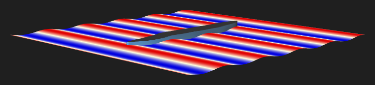
Here only the first 7 columns are shown, and we can see that the only parameter that is not close to nought is heave. This makes sense, because ship initial position is higher that the draught and it submerges until the equilibrium is reached. We can verify our conclusions by visualising the current simulation state with vtestbed-gui(1) command: all we have to do is to add (set-testbed! vtb) to the end of the script and run it.

$ vtestbed-gui sim1.scm

After that the window will appear on the screen.

This visualisation concludes the tutorial.

This video demonstrates performance increase when using graphical accelerator for computations.